At journal club, we discussed the discovery of two new hot Jupiters using data from ESA‘s CoRoT mission, with the names CoRoT-28 b and -29 b. Both systems seem a little off.
The host star CoRoT-28 has an inflated radius, suggesting it is ancient and on its way off the main sequence. But it has a lot more lithium than we’d expect for an old star, and its rotation rate is similar to the Sun’s, much faster than we would expect.
Equally puzzling is the transit light curve for CoRoT-29 b (shown below at left). Most transit curves are u-shaped, but CoRoT-29 b’s is strangely asymmetric. The asymmetry resembles what has been seen for a planet transiting a rapidly rotating star — rapid rotation reduces the gravity at the stellar equator, resulting in a cooler, darker region. Barnes et al. (2013) looked at the transit light curves for such a Kepler system and actually used the light curve to study the planet’s orbital inclination.
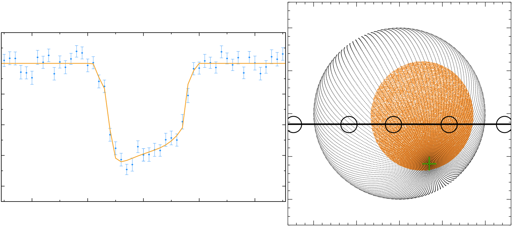
(left) CoRoT-29 b transit light curve. (right) Planet transiting star spot.
But CoRoT-29 doesn’t appear to be a rapid rotator. So instead Cabrera et al. suggest that perhaps the star has a large, nearly stationary star spot and that the planet transits the spot over and over again. However, this scenario would require a nearly stationary spot with a very long lifetime (~90 days), neither of which is expected.
So a few more astrophysical conundra to add to the growing list of puzzling exoplanet discoveries.
Journal club attendees included Jennifer Briggs, Emily Jensen, and Hari Gopalakrishnan.


