Data Science

A preliminary investigation showed a project a colleague and I were considering probably isn’t worth doing. But for that investigation, I took a few hours to make a rather complicated plot using pylab, so I thought I’d share how I did that.

First, here’s the plot:

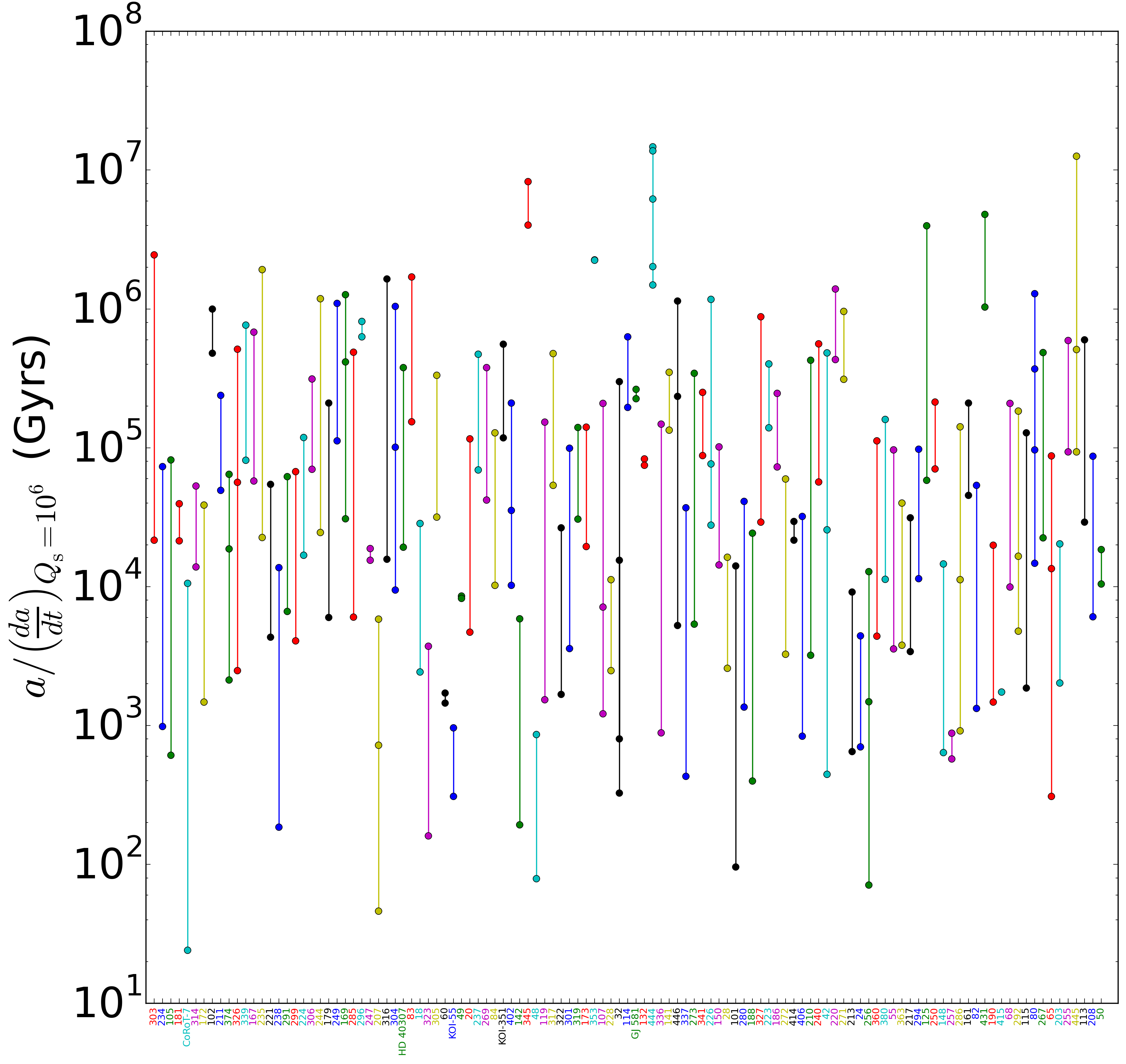
Tidal decay timescales for members of multi-planet systems.

Tidal decay timescales for members of multi-planet systems.

The plot shows the timescales for tidal decay of members of multi-planet systems. Unfortunately, the x-axis labels aren’t legible unless you zoom in, but if you do, you can see the font colors match up with the corresponding line colors.

Below is the ipython notebook I used to generate the plot. The excel spreadsheet with the data is here.

#Show the plot inline
%matplotlib inline

#load in the required modules
import pandas as pd
import pylab as pl
import itertools as it
import numpy as np

# using the ExcelFile class
xls = pd.ExcelFile('exoplanet-archive_2015Mar25.xlsx')
data = xls.parse('obj of interest', index_col=1)
data = data[pd.notnull(data['a/(da/dt)Qs=1e6 (Gyrs)'])]

#Make a nice, big figure
fig = pl.figure(figsize=(15,15))
ax = fig.add_subplot(1, 1, 1)

#Make a list, indexing the dataframe labels
indices = range(len(set(data.index)))

#Make a list with the indices as the entries
labels = list(set(data.index))
#For concision, drop "Kepler" wherever it's found
labels = [w.replace('Kepler-', '') for w in labels]

#Make a cycle of line and text colors, blue, green, red, etc.
colors = it.cycle(['b', 'g', 'r', 'c', 'm', 'y', 'k'])

#Since each member of the multi-system should be plotted with the same x-value,
#  I need to generate a new list of all the same value with as many entries
#  as members. That's what "i" is for.
i = 0
for unq in set(data.index):

    #Retrieve the decay timescales calculated in the spreadsheet
    taus = data.loc[unq, 'a/(da/dt)Qs=1e6 (Gyrs)']

    #Generate the list of all the same x-value
    idx = np.ones_like(taus)*i

    #Make the scatter plot points with the current color
    ax.semilogy(idx, taus, marker='o', color=cur_color)

    
    #Get the next line color
    cur_color = next(colors)
    
    #Next x-value
    i += 1
    
#Give a little space to the left and right of the first and last x-values
pl.xlim([-1, len(set(data.index))+1])

#Switch out the x-values with the system names
pl.xticks(indices, labels, rotation='vertical', size='small', ha='center')

#Increase the size of the y-axis label font
pl.yticks(size=36)
#Label the y-axis
pl.ylabel('$a/\\left(\\frac{da}{dt}\\right)_{Q_{\\rm s} = 10^6}$ (Gyrs)', fontsize=36)

#Reset the colors cycle
colors = it.cycle(['b', 'g', 'r', 'c', 'm', 'y', 'k'])

#Set a new color for each x-axis label
for tick in ax.xaxis.get_ticklabels():
    tick.set_color(cur_color)
    cur_color = next(colors)

pl.savefig('Comparing multi-planet system a_dadt.png', bbox_inches='tight', orientation='landscape', dpi=250)


Another attempt at using Gaussian processes to model time series, I’m looking at light curves from active galactic nuclei (AGN). The key thing I’m trying to do here is find and model flaring events.

First, I was interested to see if I could spot outliers representing the peaks of flares, while using a Gaussian processes (GP) model for background variability. The document below shows that attempt. The red band in each plot shows the GP prediction if there were no significant outliers, while the red dots show the outliers. (BTW, the way I embedded the code is very klunky but explained here.)

[gview file=”http://www.astrojack.com/wp-content/uploads/2015/03/looking_for_outliers.pdf”]

Next, I wanted to try to fit one of the apparent flaring events with a model that allowed for correlated noise. To that end, I adapted the example from Foreman-Mackey’s george python module. My solution is shown below. I need to incorporate a variable number of flaring events (I only allowed one for this example), but the model fit worked pretty well. In the second plot below, the blue band shows the range of model fits from the Markov-Chain Monte-Carlo (MCMC) analysis.

[gview file=”http://www.astrojack.com/wp-content/uploads/2015/03/fit_using_GP.pdf”]

Trying again to dip my toes into advanced data science, I decided to experiment with the Gaussian processes module in sci-kit learn. I’ve been working with barometric data to study dust devils, and that work involves spotting short dips in otherwise slowly varying time series.

In principle, Gaussian processes provides a way to model the slowly varying portion of the time series. Basically, such an analysis assumes the noise infesting each data point depends a little bit on the value of other nearby data points. The technical way to say this is that the covariance matrix for the data stream is non-diagonal.

So I loaded one data file into an ipython notebook and applied the sci-kit learn Gaussian processes module to model out background oscillations. Here’s the notebook.

In [32]:
%matplotlib inline
#2015 Feb 15 -- A lot of this code was adapted from 
#  http://scikit-learn.org/stable/auto_examples/gaussian_process/plot_gp_regression.html.

import numpy as np
from sklearn.gaussian_process import GaussianProcess
from matplotlib import pyplot as pl
import seaborn as sns
import pandas as pd
sns.set(palette="Set2")

#from numpy import genfromtxt

my_data = np.genfromtxt('Location-A_P28_DATA-003.CSV', delimiter=',', skip_header=7, usecols=(0, 1), names=['time', 'pressure'])

X = np.atleast_2d(np.array(my_data['time'])[0:1000]).T
y = np.atleast_2d(np.array(my_data['pressure'])[0:1000]).T
y -= np.median(y)

# Instanciate a Gaussian Process model
gp = GaussianProcess(theta0=1e-2, thetaL=abs(y[1]-y[0]), thetaU=np.std(y), nugget=1e-3)

# Fit to data using Maximum Likelihood Estimation of the parameters
gp.fit(X, y)

# Make the prediction on the meshed x-axis (ask for MSE as well)
y_pred, MSE = gp.predict(X, eval_MSE=True)
sigma = np.sqrt(MSE)

data = pd.DataFrame(dict(time=X[:,0], pres=y[:,0]))
sns.lmplot("time", "pres", data=data, color='red', fit_reg=False, size=10)

predicted_data = pd.DataFrame(dict(time=X[:,0], pres=y_pred[:,0]))
pl.plot(X, y_pred, color='blue')
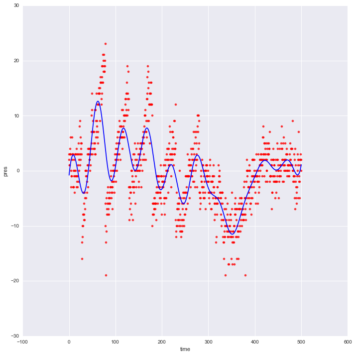
Barometric time series. Pressure in hPa, and time in seconds.

Barometric time series. Pressure in hPa, and time in seconds. The red dots show the original data, and the blue line the fit from the Gaussian process.

Unfortunately, the time series has some large jumps in it, and these are not well described by the slowly varying Gaussian process. What causes these jumps is a good question, but for the purposes of this little analysis, they are a source of trouble.

Probably need to pursue some other technique. Not to mention that the time required to perform a Gaussian process analysis scales with the third power of the number of data points, so it will get very slow very fast.

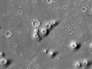
A field of pitted cones in Utopia Planitia on Mars, as observed by the HiRISE instrument onboard the Mars Reconnaissance Orbiter. Taken from http://beautifulmars.tumblr.com/post/82817530060/field-of-cones-in-utopia-planitia.

A field of pitted cones in Utopia Planitia on Mars, as observed by the HiRISE instrument onboard the Mars Reconnaissance Orbiter. Taken from http://beautifulmars.tumblr.com/post/82817530060/field-of-cones-in-utopia-planitia.

A visit from a planetary sciences colleague this weekend got me excited again about automated feature identification for remote-sensing imagery. This colleague and I talked about her work on Martian pitted cones (examples shown at left). These small hills form when a basalt flow passes over volatile (i.e., water) deposit, heating it and producing a steam explosion that uplifts the flow into a cone shape with a crater at the apex.

As for the vast majority of geomorphological studies, pitted cones on Mars are identified by groups of dedicated researchers, sifting by hand through hundreds or thousands of high-resolution images. If, instead, identification could be automated, it would help realize dramatic savings in person-hours and probably significantly increase the number of known features. It could also mitigate potential observational biases introduced by human image processing.

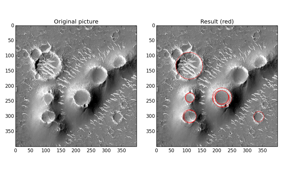
As an experiment, I applied algorithms from the scikit-image python package to find pitted cones in the example image shown at left. Fortunately, the documentation already provides a good example of circular feature detection.

So modifying the example code, I applied it to a small portion of the example image, and the figure below shows the results. Here I’m just showing the top ten most strongly detected circular features.

Unfortunately, the algorithm is not perfect — some of the obvious cones were not picked out, and others were highlighted more than once. But overall, not terrible, considering it took me about an hour and a half to implement (which included upgrading to Python 3 via the Anaconda package because scikit-image wouldn’t work with the Enthought Python version 2.7 — this upgrade will probably adversely affect my ability to use astroml, by the way).

Possible ways to improve things:

  1. The example code only returns the top two most strongly detected features for each circle radius it tries; this restriction would be simple to remove.
  2. The fact that the pitted cones are cone-shaped means you could require that any putative crater be framed by an appropriately shaped shadow. Regardless of the cone’s actual height (probably unknown anyway), the shadow on the cone should darken as the solar incident angle approaches 180 degrees, modulo any nearby morphological features (as evident in the figure below).
My attempt to automatically identify pitted cones using scikit-image.

My attempt to automatically identify pitted cones using scikit-image.

As part of my new push into data science, I read Shi & Malik’s paper on the perceptual grouping problem in which they develop a new algorithm for dividing an image up into coherent regions.

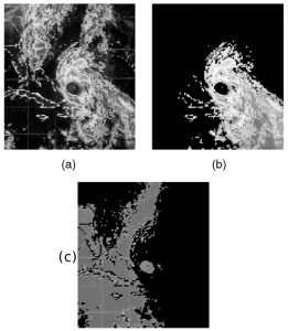
A portion of Figure 8 from Shi & Malik (2000).

A portion of Figure 8 from Shi & Malik (2000).

What does it mean to divide an image into coherent regions? Say, for example, you had a satellite image of a large storm system, such as the figure at left from Shi and Malik’s paper. Panel (a) shows the original image, while (b) and (c) show two portions of the image grouped together by Shi and Malik’s algorithm. The result makes intuitive sense (at least, to me): (b) is a large part of the storm, while (c) is the ground underneath.

Basically, Shi and Malik’s algorithm treats the entire image as a weighted graph, with portions of the image treated as nodes. Weights on the edges connecting the nodes are larger for portions that are closer to each other and for portions that are similar (where similarity may depend on the pixel brightnesses, textures, colors, etc.).

The algorithm decides which portions belong together as one segment using the weights for all the nodes connected in that segment. Shi and Malik developed a clever way to turn this process into an eigenvalue/vector problem, thereby dramatically facilitating the calculation. Their technique amounts to treating the pixels as individual masses connected by springs, with spring constants given by the edge weights, and then finding the normal modes of oscillation for the system: pixels that are strongly coupled are grouped together as one segment.

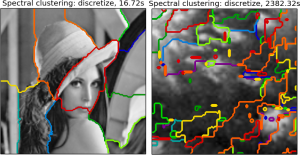
Conveniently, the algorithm is implemented in the scikit-learn python module. Using their example code, I was able to reproduce the segmentation of the Lena image easily (shown below), so I thought to try it on some VIMS observations of Titan. (Here’s the original Titan image. I took a small portion of it.)

Unfortunately, the result was not promising: the algorithm did NOT break up the image into the segments I expected. Instead, the segments seem pretty random. It also took about 40 minutes to work, even though the Titan image is smaller than the Lena image (100 x 100 pixels vs. 128 x 128).

(Left) Result from the spectral clustering example code on the scikit-learn page. (Right) My own attempt at segmenting a VIMS image of Titan.

(Left) Result from the spectral clustering example code on the scikit-learn page. (Right) My own attempt at segmenting a VIMS image of Titan.

Next things to try: it seems the algorithm needs me to tell it how many regions to use — I used the number given in the original example, 11. Maybe I should try a smaller number. There are also a few options as to how the graph weight are calculated in the original Shi and Malik algorithm (not sure if the scikit-learn module has that capability).