Data Science

UPDATE (2018 Jun 6) – I’m trying to learn how to use Sphinx to create documentation from source-code docstrings. The Sphinx manual is impressively opaque. Some googling turned up this document, which seems to provide useful details.

UPDATE (2018 Jun 4) – I’ve found some new resources that are much more up-to-date:

To set up my package so it can be installed via pip, I’m following the somewhat outdated tutorial here – https://python-packaging.readthedocs.io/en/latest/index.html.

I’ll make more notes and update this post as I go along.

As the second entry in my series on learning how to write scientific software, I’m going to describe choosing and configuring my integrated development environment or IDE. This is the program I’ll use to write and edit the source code for my project. It’s more-or-less a fancy text editor.

My text editor of choice is vim or vi improved. It’s highly customizable, powerful, and there’s lots of online help to use it. However, it has a very steep learning curve and the commands, while fast to type out, can be very cryptic. In fact, vim is famously difficult to exit.

In any case, I started using vim back when “Pirates of the Caribbean” movies were still good, so while I’m no vim guru, I feel pretty comfortable at least exiting the program.

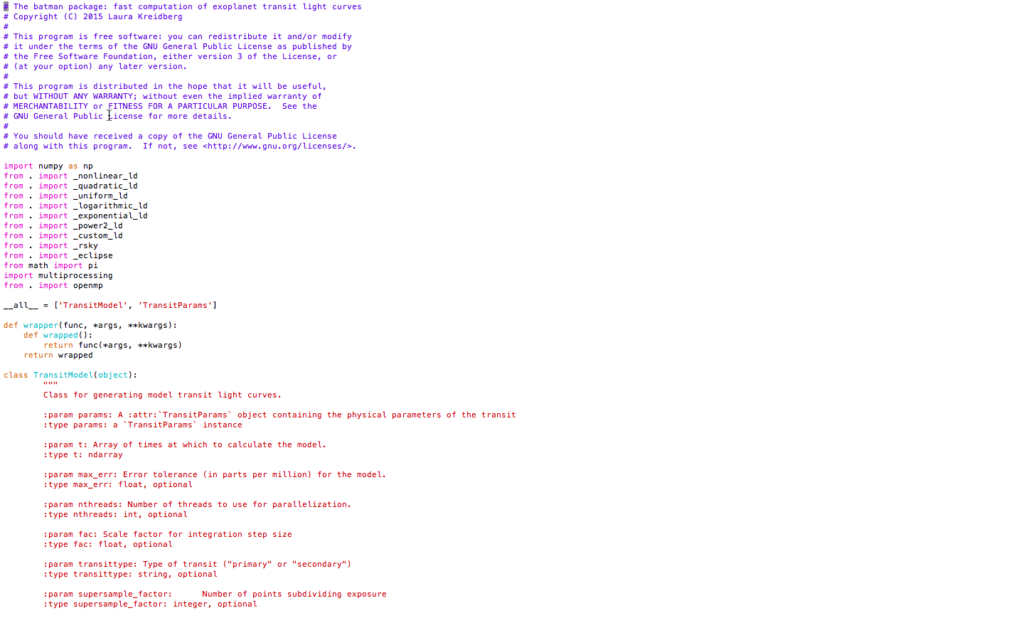
Opening a terminal window in Mac, I fire up vim just by typing “vim” or “vi”. That opens an editor window. vim can automagically interpret and color source code, as follows:

A screenshot from vim showing syntax-colored source code.

To turn on syntax coloring, go to your home directory (type “cd” in the terminal window), and edit the vim configuration file .vimrc by typing “vi .vimrc”. That should open an editor window.

Then, in vim, type the letter “i” (that starts “insert” or edit mode, allowing you to enter text into the file) and type “syntax on” <ENTER> “filetype indent plugin on”, giving a file that looks like this:

Press the escape key (which exits insert mode and enters command mode). Save the changes by typing “:wq”. That should save and exit.

Unlike many other languages, Python considers whitespace in its interpretation, and the Python style guide recommends using four spaces for each level of indentation. It would be nice to have the tab key implement that spacing in vim. Ynfortunately, my vim by default inserts eight spaces for each press of the tab key.

But you can modify that behavior by adding file-type plugin files to a special vim configuration folder. I followed the instructions here to create an ftplugin directory inside the .vim directory (by typing “cd && cd .vim && mkdir ftplugin && cd ftplugin” in the terminal window). Then, inside the directory, I created python.vim (“vi python.vim”) and again pressed “i” to enter insert mode.

I typed the following lines into the file:

Then pressed the escape key and typed “:wq”.

Next, I tested the new configuration by typing “vi test.py” (the “.py” is important because that’s how vim knows you are editing a python file and want to use the new python configuration). I pressed tab and got four spaces instead of eight.

I’m sure there are other configuration settings that would be useful, but this’ll do for now.

UPDATE – 2018 May 17: I found this excellent website – http://docs.python-guide.org/en/latest/, which addresses vim set-up, as well as a number of other issues.

Ancient software developers meticulously punched holes in paper cards to write programs.

In the eons before my graduate career, scientists rarely, if ever, publicly distributed their codes, with authors zealously guarding their coding projects.

But just as I was finishing my PhD, it was becoming common for scientists to make the code they developed as part of a published project readily available on the internet. However, the methods to post code online (at least those I knew about) were pretty clunky.

Nowadays, the infrastructure for posting and sharing code online is robust, mature, and relatively easy to use. Consequently, scientists are creating beautiful code repositories, along with accessible documentation.

Open-sourcing code is becoming ever more important: as codes become more complex and capable, readily available codes with good documentation are critical to support reproducibility, a cornerstone of the scientific process. Moreover, federal funding agencies are starting to require investigators to make their code and data products public.

Unfortunately, since I was one of the last generation of grad students before these repositories were common, I never really learned how to distribute and document code properly.

So as part of an ongoing effort to improve my science output (and as an aide to my future students), I’m going to begin a series of semi-regular blog posts describing my process of learning how to write, document, and post scientific code.

A few caveats upfront:

  • I intend to mostly (probably exclusively) write the code in python, which has become (at least in astronomy) the language of choice, so not all of what I write will be generally relevant.
  • I was ushered into the Cult of Mac many years ago, so not all of what I write will be relevant for other OS’s. Here again, though, I’ve found anecdotally that most astronomers use Mac.
  • This blog series is in no way intended to be comprehensive or rigorous. I’m just planning to describe what I learn as I go along, and what time I can devote will almost definitely not suffice to explain all the details, nuances, or technical aspects that intersect the project.

As to the actual science code I intend to write, several years ago my colleagues and I wrote a paper about ellipsoidal variations induced by massive exoplanets orbiting very close to their host stars. The accompanying code, EVIL-MC was written in IDL, an older language still widely used in astronomy but proprietary and requiring the purchase of an expensive site license.

My plan is to convert that IDL code into a Python package over the next several weeks.

EVIL-MC – Ellipsoidal Variations Induced by a Low-Mass Companion


Tidal distortion (exaggerated) of a star (orange-yellow disk) orbited by planet (white/black disk). The plot below shows the brightness variation of the star due to the tidal distortion.

OCR OC-gain

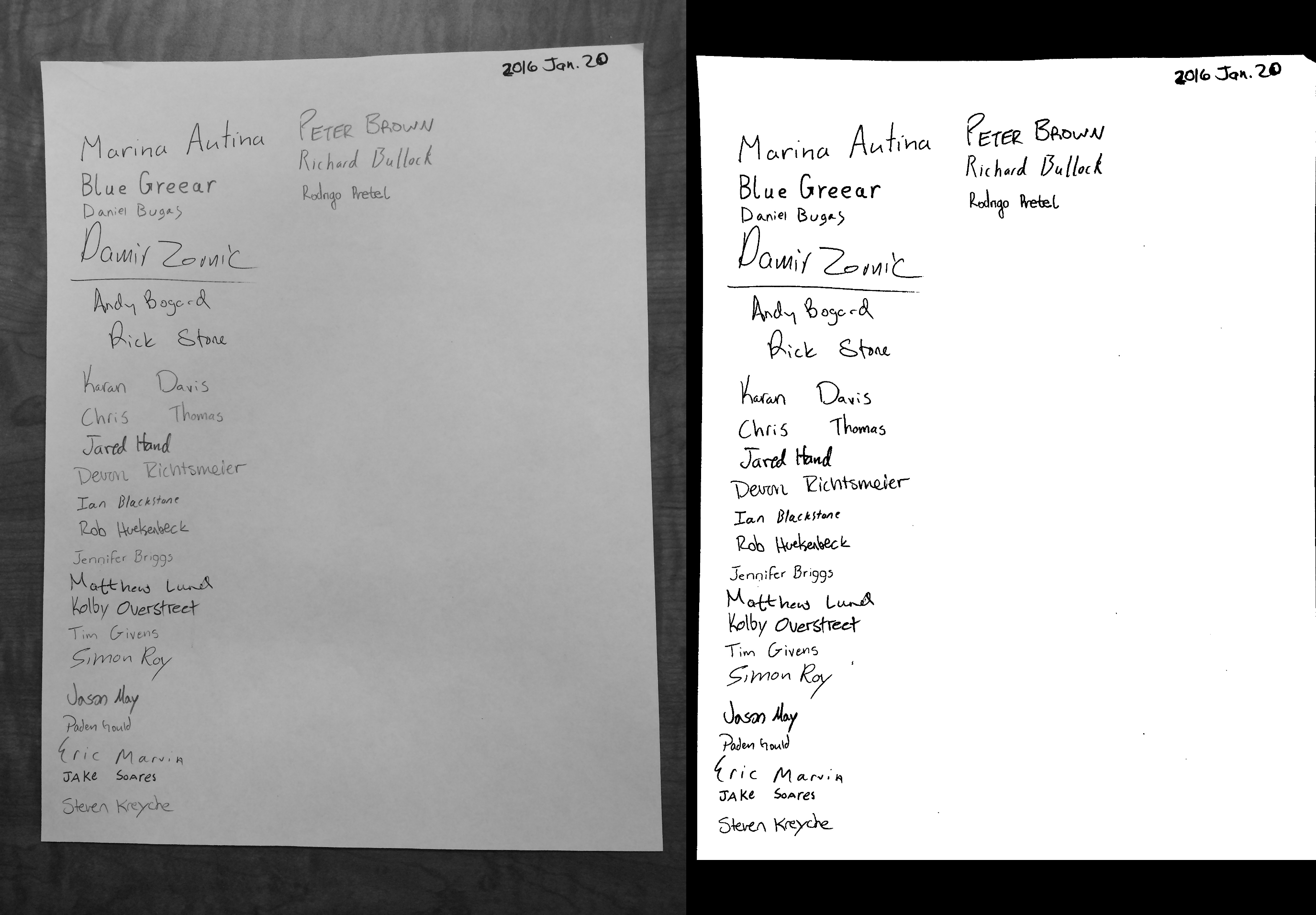
My PHYS341 students were interested to see how the OCR routine processed their attendance sheet, so I applied it, as shown below.

IMG_3707_orig-scannedThe left panel shows the original, the right the transformed version. The routine did a reasonable job of un-distorting the page (although it wasn’t too bad to begin with).

And here’s what the routine returns as text:

zolto J:)o<-&\
Qfick ${‘bt\L . .
1ZWrW(\ DQVCS
Onras Tkomag
Jam; I-Em!
De»-UV1, ?I‘L\M‘ovV\QJ3€,v'
Ia./I B,a,C/IHMC .
V.o\3 \3<<I°\Ser&eck
jengifcr Brigga
}VK°'('3E\V1c-rad LULAA
Mby Ouersfreci’ '
Tm (jivws ‘
gj)/VIOI/I  ‘
$030-4 “10u\J ‘
{NC /I/1a.V,,,,',q '
O”AKe So/ares
Skwm \<reyc}~e '

…not great.

I’m not totally sure what went wrong. Maybe I should have them write their student numbers instead.

UPDATE: 2016 Feb 5

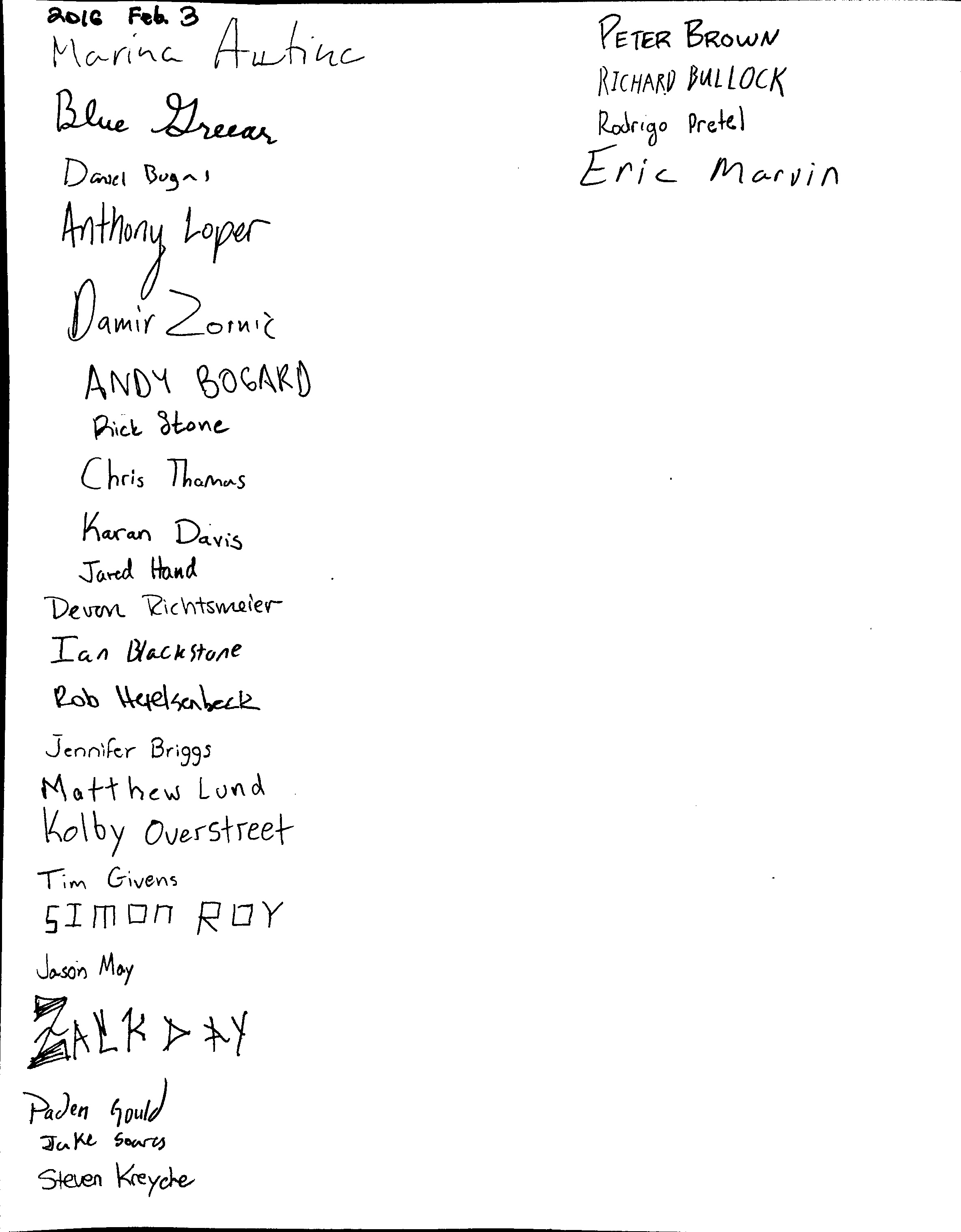
Here’s another go with a different attendance sheet. Not much better.

IMG_3784_scanned

I‘/\0,;/{¢r\(~  VETEK BROWN
E ? RICH/W} WLMC/(
“$2114!/~, lZoAr.‘%o Pratt.‘
D“""‘ 8'3"’ ' g/"It; /Vlar,//'/1
 Lolpef‘
kpdkl/n\‘f 2011/(IE
ANN <5©<J\M) Vfxit %'L0V\€z &}"-:5 _)_La/\/MAS _ Karm I>q'v‘-5
\Tou—o0l Hand _
'Dz\m/L ?\c\n'ksvvuu‘ev*
Ian I3/¢«'-Ckfia/If ¢
94% \5<<k*?l6<:x\.cLl¢ Jennifer BH995 N\o+‘\'V\c\.6 Luv\0\ . \/\0\\)y 0\,ers+reeJr ’\".m C"\\/Ens _ 51 m cm E 1: Y Jason May A ZPM > M
PIJW1 figu//
jam 5°0W'/J
34681 \4'€y¢}~¢>/

I spent the morning kludging together a python script to convert a grocery receipt into a spreadsheet as part of one of my New Year’s resolutions. There seem to be a few options out there for scanning and recording receipts, but it’s not clear that they apply an OCR technique to automatically convert them to spreadsheet.

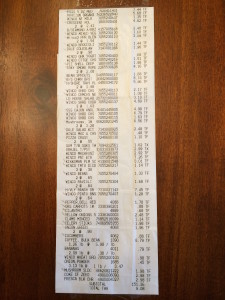
Here’s the receipt I used:

IMG_3497This website provided some python source code to detect edges in the image then the outline of the receipt and transform out any foreshortening or other viewing distortion —

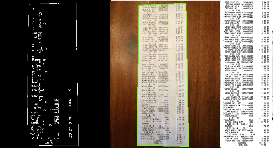
(left) Edge detection, (center) Outline detection, (right) Scanned version.

(left) Edge detection, (center) Outline detection, (right) Scanned version.

To detect edges, the code converts the color image to grayscale and applies the Canny edge detection scheme, which involves applying a Gaussian blur to suppress noise, calculating image derivatives, and looking for large values. The result is shown in the image above on the left, and more details on the algorithm here.

Next, the code finds the outline of the receipt by using the OpenCV‘s findContours, sorts the contours by area, and finds the contour with the largest area but with four vertices.

The code then applies a four-point transformation to warp the receipt to give it a rectangular shape and finally thresholds the grayscale to enhance the contrast. The rightmost panel in the above image shows the final result.

To convert the image to a table of text, I used PyTesseract, which provides OCR capabilities. I installed the package Tesseract using homebrew: “brew install tesseract”.

Then I just grabbed the code from this website to convert the final result into a text table:

st = pytesseract.image_to_string(Image.open(save_filename), config="-psm 6")

The “psm=6” option was required to return the text properly.

Unfortunately, the OCR analysis wasn’t perfect. For example,
IMG_3497_scanned_linewas converted to
‘*CRESgENT R01 1 1800000401 4.82 IF

The prices on all lines came back fine, but the description was often distorted. I decided I cared more about the price anyway. Fortunately, the WinCo receipt had “TF” or “TX” at the rightmost side, so I performed a regex search to find the beginning of that string and grabbed the characters to the left of that.

Finally, I converted the strings into a list of comma-separated values to load into Excel or Google Sheets, leaving a space between the corrupted description and price so I could enter my own description, giving
CRESgENTR0111,  , 4.82

On the off-chance it will be useful to someone else, I’ve posted the code here. Using my script will also require the source code for pyimagesearch, which requires submitting an e-mail address.

As part of a project, I’m trying to learn how to do motion capture on videos. Fortunately, there’s Python support for the OpenCV computer vision library.

I adapted some motion capture code I found online that uses the Shi-Tomasi Corner Detector scheme to find good features to track — regions in a grayscale video frame that have large derivatives in two orthogonal directions.

Then the code estimates the optical flow using the Lucas-Kanade method, which applies a least-squares fit to solve for the two-dimensional velocity vector of the corner features.

As a test case, I used a video of Alice singing the “Ito Maki Maki” song.

The shiny tracks in the video show the best-fit model. Interestingly, the corner detection scheme chooses to follow the glints in her eyes and on her lip. The motion tracker does a good job following the glints until she blinks and swings her arm across her face.

The code I used is posted below.

import numpy as np
import cv2
cap = cv2.VideoCapture('IMG_0986.mov')
size = (int(cap.get(cv2.cv.CV_CAP_PROP_FRAME_WIDTH)),
int(cap.get(cv2.cv.CV_CAP_PROP_FRAME_HEIGHT)))

# params for ShiTomasi corner detection
feature_params = dict( maxCorners = 100,
qualityLevel = 0.3,
minDistance = 7,
blockSize = 7 )

# Parameters for lucas kanade optical flow
lk_params = dict( winSize = (15,15),
maxLevel = 2,
criteria = (cv2.TERM_CRITERIA_EPS | cv2.TERM_CRITERIA_COUNT, 10, 0.03))

# Create some random colors
color = np.random.randint(0,255,(100,3))

# Take first frame and find corners in it
ret, frame = cap.read()
old_gray = cv2.cvtColor(frame, cv2.COLOR_BGR2GRAY)
p0 = cv2.goodFeaturesToTrack(old_gray, mask = None, **feature_params)

# Create a mask image for drawing purposes
mask = np.zeros_like(frame)

images = list()

height , width , layers = frame.shape

fourcc = cv2.cv.CV_FOURCC('m', 'p', '4', 'v')
video = cv2.VideoWriter()
success = video.open('Alice_singing.mp4v', fourcc, 15.0, size, True)

ret = True
while(ret):
  print(ret)

  frame_gray = cv2.cvtColor(frame, cv2.COLOR_BGR2GRAY)

# calculate optical flow
  p1, st, err = cv2.calcOpticalFlowPyrLK(old_gray, frame_gray, p0, None, **lk_params)

# Select good points
  good_new = p1[st==1]
  good_old = p0[st==1]

# draw the tracks
  for i,(new,old) in enumerate(zip(good_new,good_old)):
    a,b = new.ravel()
    c,d = old.ravel()
    cv2.line(mask, (a,b),(c,d), color[i].tolist(), 2)
    cv2.circle(frame,(a,b),5,color[i].tolist(),-1)

  img = cv2.add(frame,mask)

  video.write(img)
  ret,frame = cap.read()

# Now update the previous frame and previous points
  old_gray = frame_gray.copy()
  p0 = good_new.reshape(-1,1,2)

cap.release()
video.release()
cv2.destroyAllWindows()

With the help of physics major Jared Hand, we’ve started a weekly meeting group here in physics to discuss scientific computing — the Boise State SciComp Workshomp.

The meetings take place in the physics building, room MP408, and will focus on the nitty gritty of scientific computing — how to install and run various codes and packages.

We’ve started a github repository for the group: https://github.com/decaelus/BoiseState_SciComp_Workshomp.

We will keep a log of our meetings on the associated wiki: https://github.com/decaelus/BoiseState_SciComp_Workshomp/wiki/Working-with-Git.

We’re currently working through a presentation from the Software Carpentry Foundation on using git: http://slides.com/abostroem/local_version_control#.

github-octocatHad our first Scientific Computing Discussion group meeting on Friday at noon. These meetings are intended to familiarize our students with scientific computing applications and how to manage and maintain various science computing modules. We started a github repository where we’ll post notes and other information: https://github.com/decaelus/BoiseState_PAC_Workshop.

Attendees included Liz Kandziolka, Emily Jensen, Jennifer Briggs, Ahn Hyung, Tiffany Watkins, Jesus Caloca, and Helena Nikolai. Jared Hand helped lead the discussion. (Apologies to those of you who attended but I didn’t record your name.)

From http://en.wikipedia.org/wiki/Reese%27s_Pieces#/media/File:Reeses-pieces-loose.JPG.

From http://en.wikipedia.org/wiki/Reese%27s_Pieces#/media/File:Reeses-pieces-loose.JPG.

I eat Reese’s pieces almost every day after lunch, and they come in three colors: orange, yellow, and brown.

I’ve wondered for a while whether the three colors occur in equal proportions, so for lunch today, I thought I’d try to infer the occurrence rates using Bayes’ Theorem.

Bayes’ Theorem provides a quantitative way to update your estimate of the probability for some event, given some new information. In math, the theorem looks like

$latex P\left( H | E \right) = \dfrac{ P\left( E | H \right) P\left( H \right)}{P\left( E \right)},$

The probability for event $latex H$ to happen, given that some condition $latex E$ is met, is the probability that $latex E$ is met, given that $latex H$ happened, times the probability for $latex H$ to happen at all, and divided by the probability for $latex E$ to be met at all.

The $latex P(H)$ and $latex P(E)$ are called the “priors” and often represent your initial estimates for the probability that $latex H$ and $latex E$ occur. $latex P\left(E | H \right)$ is called the “likelihood”, and $latex P(H | E)$ is the “posterior”, the thing we know AFTER $latex E$ is satisfied. $latex P(H | E)$ is usually the thing we’re trying to calculate.

Big bag

Thanks, Winco buy-in-bulk!

So for my case, $latex P(H)$ will be the frequency with which a certain color occurs, and $latex E$ will be my experimental data.

For a given frequency $latex f_{\rm orange}$ of oranges (or browns or yellows), the probability $latex P(f_{\rm orange} | E)$ that I draw $latex N_{\rm orange}$ oranges is  ~ f^N (1 –  f)^N(not orange). As I select more and more candies, I can keep re-evaluating $latex P$ for the whole allowed range of f (0 to 1) and find the value that maximizes $latex P$.

Closing my eyes, I pulled ten different candies out of the bag, with following results in sequence: brown, orange, orange, yellow, orange, orange, orange, brown, orange, yellow, orange. These results obviously suggest orange has a higher frequency than yellow or brown.

This ipython notebook implements the calculation I described, and the plots below show how $latex P$ changes after a certain number of trials $latex n_{\rm trials}$:
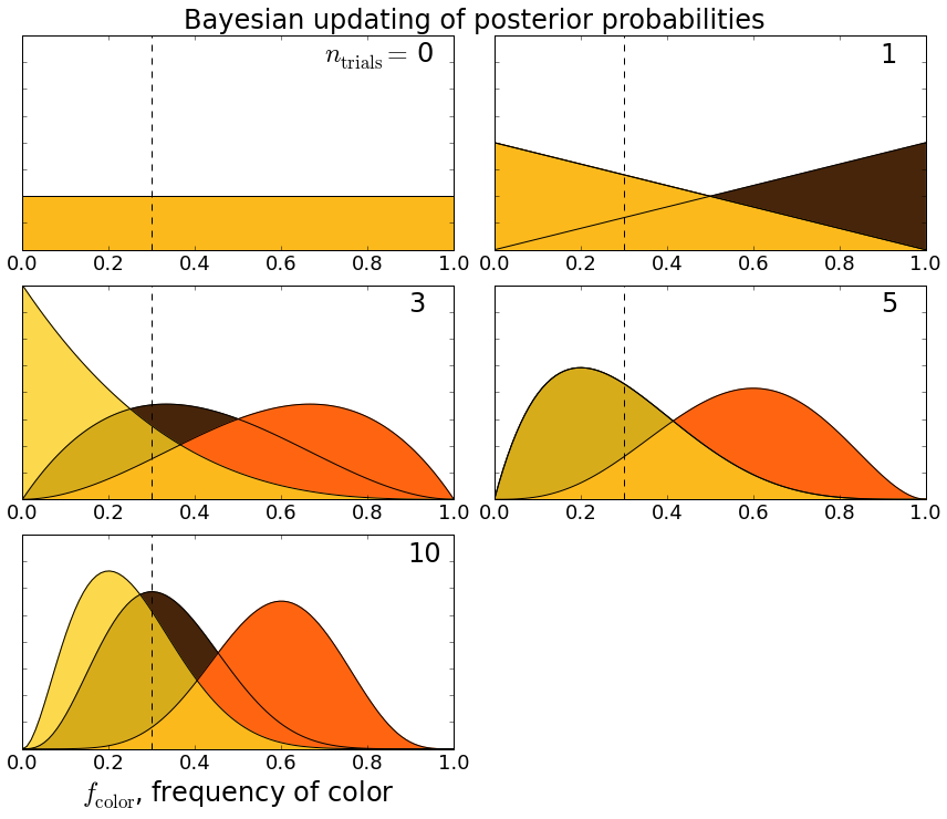
Applying Bayesian inference to determine the frequency of Reese's pieces colors.

Applying Bayesian inference to determine the frequency of Reese’s pieces colors.

So, for example, before I did any trials $latex n_{\rm trials} = 0$, I assumed all colors were equally likely. After the first trial when I chose a brown candy, the probability that brown has a higher frequency than the other colors goes up. After three trials (brown, orange, orange), orange takes the lead, and since I hadn’t seen any yellows, there’s a non-zero probability that yellow’s frequency is actually zero. We can see how the probabilities settle down after ten trials.

Based on this admittedly simple experiment, it seems that oranges have a frequency about twice that of yellows and browns. Although not as much fun, if I’d bothered to check wikipedia, I would have seen that “The goal color distribution is 50% orange, 25% brown, and 25% yellow” — totally consistent with my estimate.